Welcome to a journey into our Universe with Dr Dave, amateur astronomer and astrophotographer for over 40 years. Astro-imaging, image processing, space science, solar astronomy and public outreach are some of the stops in this journey!
Full “Wolf” Moon captured on the eve of 1/27 from Mayhill NM. The halo around the Moon is an indication wet or stormy weather is imminent according to the Old Farmer’s Almanac
Typically a full moon and the few days before and afterward mean no imaging or observing during that period, at least for me! Don’t get me wrong though. I distinctly remember the first time I saw a full moon here in the Desert Southwest. It was truly amazing! With no surrounding trees or other obstructions it seemed as bright as day. The mountains in the distance could easily be seen. An eerie but peaceful glow was cast over the desert as far as you could see. For many folks the full Moon is really something to observe and not just an inconvenience. It’s obviously the easiest object in the night sky to see! I occasionally am asked by someone “Did you take pictures of the Flower Moon last night?” or the Corn Moon, or the Buck Moon etc etc. Of course I’m not going to image the Moon , not counting the iPhone image above, when it’s full unless it’s being eclipsed by the Earth’s shadow 🙂 However these questions did pique my interest in this “Moonlore” everyone seems to know about except me. I know about Harvest Moon and of course “Blue Moon” when you have two full moons in the same month but most of these other names I am completely unfamiliar with. So I decided now was the time to give the Full Moon its’ due and let’s see what this mystique is that has been built around it.
“The Moon names come from Native American, Colonial American, or other traditional North American sources passed down through generations. Note that for Native American names, each Moon name was traditionally applied to the entire lunar month in which it occurred, the month starting either with the new Moon or full Moon. Additionally, a name for the lunar month might vary each year or between bands or other groups within the same nation. Historically, names for the full or new Moons were used to track the seasons. Think of them as nicknames. Many of the names are English interpretations of the words used in Native American languages.” (courtesy Almanac.com)
“The early Native Americans did not record time by using the months of the Julian or Gregorian calendar. Many tribes kept track of time by observing the seasons and lunar months, although there was much variability. For some tribes, the year contained 4 seasons and started at a certain season, such as spring or fall. Others counted 5 seasons to a year. Some tribes defined a year as 12 Moons, while others assigned it 13. Certain tribes that used the lunar calendar added an extra Moon every few years, to keep it in sync with the seasons.” (almanac.com)
Today is the first Full Moon of the year. It’s thought that January’s full Moon came to be known as the Wolf Moon because wolves were more often heard howling at this time. It was traditionally believed that wolves howled due to hunger during winter.
Here is a table of the Moon names and a brief description of their meaning below. Read the table from left to right for each month.
Table of full moon names (almanac.com)
February– Full Snow Moon- Refers to typically heavy snowfall during the month
March– Full Worm Moon- Named after the earthworms of warming Spring soil
April– Full Pink Moon- The color of wild ground Phlox, a pink Spring wildflower
May– Full Flower Moon- Abundance of flowers in this month
June– Full Strawberry Moon- Ripening strawberries in the Northeast US
July– Full Buck Moon- A buck’s antlers are in full growth
August– Full Sturgeon Moon- The Sturgeon of the Great Lakes in the US are abundant this month
September– Full Corn Moon, OR Harvest Moon: “According to one tradition, which the Old Farmer’s Almanac honors, the Harvest Moon is always the full Moon that occurs closest to the September equinox. Most years, it falls in September; every three years, it falls in October. (Astronomical seasons do not match up with the lunar month.) If the Harvest Moon occurs in October, the September full Moon is usually called the Corn Moon instead. Similarly, the Hunter’s Moon always follows the Harvest Moon. (Note that these last two conditions are not according to Native American tradition.)” (courtesy Almanac.com)
October– Full Hunter’s Moon- Time for hunting and gathering provisions for the long months ahead
November– Full Beaver Moon- Beavers finish preparations for Winter
December– Full Cold Moon- Fairly obvious I think!
So there you have it. Moonlore galore. Enjoy the Wolf Moon tonight!
The well-known “Double Cluster” in the constellation Perseus consists of two open star clusters NGC 869 and NGC 884 (often designated h Persei and χ Persei, respectively), which are just a few hundred light years apart . Both visible with the naked eye at just under 4th magnitude, NGC 869 and NGC 884 lie at a distance of 7,500 light years from us. There are more than 300 blue-white super-giant stars in each of the clusters and NGC 884 contains 5 prominent red giant stars which also happen to be variable stars. NGC 869 appears slightly brighter, richer and more compact than NGC 884.
For the full resolution version find the link under “My astroimages” on the lower right side of this page.
NGC 884 contains 5 red giants which are numbered above. This part of the double cluster is not as compact as the lower portion NGC 869
The Perseus double cluster is easily visible to the naked eye in the Northern Hemisphere. Look slightly west of north after sunset currently . Look just below Perseus and above the constellation Cassiopeia which now looks like a “W” pointing to the right and slightly downward. Three stars of the “W” are seen at the very bottom of the image above. The cluster sits in between the two constellations (blue square in the image above)
The cluster looks tremendous in a pair of binoculars! Don’t miss it.
Last time we discussed the concept of atmospheric seeing and image scale and how your telescope camera combination yields a specific value of that image scale in arc seconds per pixel where each pixel sees a certain amount of sky. This value is fixed. What is not fixed is the sky conditions which can vary greatly.
Plot of light intensity vs width for a star. “FWHM” stands for “full width at half maximum”. The hatched line is where the star’s disc is measured typically in arc seconds
Atmospheric seeing is estimated by measuring the width of a star’s disc in a point spread function at half the star’s maximum intensity , also known as the “full width at half maximum” (FWHM). This value can be measured in arc seconds or in pixels from your specific camera. So for example let’s say your camera- telescope combo yields a scale of 3 arc seconds per pixel and the FWHM that night is 3 arc seconds. You could also say on that night that the FWHM is 1 pixel. We also discussed that we know from very smart statistical mathematicians that to get the most information from the deep space object you are interested in we want somewhere between 2 and 3 pixels to cover that FWHM. The main problem occurs when you have less than 2 pixels. This is called undersampling. In this case “supposedly” you are going to have ugly square shaped stars and blocky transitions in your images. In 20 years of imaging I never thought I had really seen this phenomenon. This kind of mismatch can happen for amateurs using wide field set-ups with smaller scopes and shorter focal lengths. To be fair I have been doing more of that recently than I ever have so perhaps that is why I haven’t come across it….until now.
Now as we also discussed last time, undersampling happens very frequently with the Hubble Space Telescope! My guess is that they don’t make pixels small enough yet to match the perfect seeing in outer space, but that’s just a guess. At any rate, undersampling is enough of a problem for them that they felt the need to figure out a solution. The solution is called drizzle integration.
“Drizzle is a digital image processing method for the linear reconstruction of undersampled images. The algorithm, known as variable-pixel linear reconstruction, or informally as “Drizzle”, preserves resolution, can weight input images according to the statistical significance of each pixel, and removes the effects of geometric distortion” (Wikipedia). Integration, for non astro-imagers, is a process where you combine your images statistically using software to enhance the image details while removing the artifacts and noise in the images. For example let’s say you are taking an image of a star cluster and you want to expose a total of about 4 hours. Instead of taking 1 exposure of 4 hours, you take many exposures of a few minutes each. By aligning the images, then statistically combining them you actually increase the resulting signal more so than a single exposure would. This is integration. The drizzle component analyzes the files and reconstructs the pixel configuration so when you integrate your images your resolution is improved compared to the undersampled result. Ok enough of this background info. Is this really true? I wanted to find out for sure. I looked back at a couple of my wide field images and ok maybe the features were a little abrupt. Maybe some areas were pixelated but this was all very subjective. The good news is that you absolutely don’t need to understand any of the statistical math involved here. There are a hundred or so software programs now for image processing where many will have drizzle integration options there. All you have to do is point and click…seriously! So now the fun begins and I will go through this for the popular processing program Pixinsight and let’s see if it really makes a difference or not.
First off we need to ask “How do I know if drizzle integration is going to help me”? The main criteria we have discussed which is that your image is of course undersampled defined as a FWHM less than 2 pixels. The other thing which is helpful in this process for drizzle to work is that your images should optimally be dithered. Ok , another weird term. Most of us during image acquisition shift each successive image slightly by around a pixel or two so that when the images are aligned during processing, only the important stuff lines up and the noise etc is not lined up, to put it in simple terms. This is “dithering”. During the statistical combine all the stuff not lined up is treated as noise and artifact and is removed because it does not occur in the same pixel location in each image, where the aligned features will be in the same location and those will be enhanced during integration. The third thing which can help is having enough images so noise is not excessive. This number turns out to be greater than about 15.
Step 1. Are we undersampled?
In Pixinsight the FWHM can be calculated very easily!
Luckily some very smart people have made this whole thing very easy for us! You don’t have to rely on the eye test to see if you’re undersampled. In the image above I have a red channel raw frame of the Perseus Double Cluster open: a perfect test for this since this is a very star-dense image. In the Pixinsight program , simply go to “scripts”> “image analysis” > FWHMEccentricity.
When you open the script, make sure your image is displayed in the drop down at the top and just click on the “measure” button at the bottom. Here the Median FWHM for the image is measured to be 1.86 pixels. Ok by definition we are undersampled here!
Step 2. Align your images and generate the “drizzle data”
Batched preprocessing script in Pixinsight showing the Image registration pane and circled checkbox for “Generate drizzle data”
Next we take our already calibrated images meaning we have subtracted the dark current and optical aberrations with flat subtraction and now we are ready to align the images, also called “image registration”. All you have to do is check the box in the image registration pane that reads “generate drizzle data”. That’s all! During the alignment process, the program will do the pixel reconstructions automatically so when you do drizzle integration everything is ready to go.
Addendum: Note that here we are using the weighted batch preprocessing script which I think is the easiest way. If you do that, integration will occur as well (note the “apply box” is checked under image integration) and will automatically update the drizzle files so you would go next to step 4 below. If you do not use the preprocessing script and use star alignment for registration as a stand alone process, then go to step 3. Hopefully that is not too confusing. I missed this point in my original post, namely that when you use the weighted batch preprocessing script as we are doing here, you do not have to reintegrate with normal integration.
Step 3. Update the drizzle files by doing “normal” integration first if you used the Star Alignment process. Otherwise go right to step 4 as explained above.
Next you integrate your files as you normally would using the standard image integration process, with one exception. After you add your files, you click on the “add drizzle files” button so in essence you are adding the files twice but the second time the drizzle info is included. You will notice that after adding the files in initially like you always do the “add drizzle files” button will become accessible. In Pixinsight the drizzle files have the extension “xdrz”. Then you integrate by clicking on the blue circle at the bottom which is the “apply all” button in Pixinsight. You will get an integrated image result which is just for reference really but we will use that to compare the result after the “drizzling” is complete!
Step 3. Drizzle integration. The moment we have all been waiting for!
After you have done the integration the usual way and updated the drizzle files as described above you will repeat the integration using the drizzle process. Drizzle integration is carried out by opening the “drizzle integration” process in Pixinsight as opposed to just “image integration” like we used above. Click on “add files” where it will automatically load the updated drizzle files from the previous integration process confirmed by the “xdrz” file extension you can see circled there. I had to fiddle figuring out the best screen shot resolution to show the difference in the stars so the file extension unfortunately is difficult to see, but you get the idea. The other settings are left alone at their default values. There is something called “scale” which is left at 2 and something called “drop shrink” which is 0.9. You don’t need to worry about any of that except to be aware that the scale of 2 means your image will wind up 4 times larger after the drizzle process is done!
I think you can see the difference in the image above pretty clearly. The star image on the right shows the integrated result without drizzle and the left with the drizzle integration. The black arrows point to the identical stars in each image. Without drizzle the star is clearly pixelated on the right where on the left it is round and smooth! The effect is much more dramatic live than in this screen shot reproduction.
Another example above of standard integration without drizzle. Notice the square pixelated stars.
Drizzle integration is again shown above. Stars are round and smooth!
I don’t know about you but I am convinced. Bottom line is for your wider field setups, check your images’ FWHM and if it is less than 2 pixels consider drizzle integration, courtesy of the Hubble Space Telescope science team!
We begin another installment on our image processing series where I review some aspect of image processing I have found interesting or intriguing and these are typically things I was not aware of previously, so it’s a learning experience on both ends! Today we will discuss some background info regarding seeing and image scale before going on to part 2 where we will explore the technique of what’s called “drizzle integration”. Sounds weird but hopefully it will become clearer as we move along.
What happens when starlight passes through our atmosphere it changes from a point source of light and becomes a disc
If you were able to observe stars from the orbiting space station, above Earth’s atmosphere, they would appear as tiny pin dots of light. When the star light travels through Earth’s atmosphere though, it unfortunately spreads out and becomes a disc. If you plot intensity of the light vs width or diameter of the disc you arrive at what is known as a “point spread function” (see below). We are at a significant disadvantage obviously being here on the Earth’s surface in terms of trying to see details in deep space objects. The same spreading out of light will occur with any object in space we are looking at but starlight being at least a point source at its origin is the easiest to measure this effect.
Plot of light intensity vs width for a star. This is what a “point spread function” looks like. “FWHM” stands for “full width at half maximum”. The hatched line is where the amount of “spreading” of the starlight is measured typically in arc seconds
This “disc” of starlight changes size all the time depending in part on how turbulent the atmosphere is. This is often referred to as atmospheric seeing. Obviously the smaller the disc the better for us. Since the atmosphere surrounding Earth is also a sphere, measurements of any object we see are typically angular in nature. For example, if you take the entire sphere of the sky measuring 360 degrees, the full Moon has a diameter of close to ½ a degree. The small stellar discs we are talking about have diameters typically of 2-4 arc seconds (60 sec in 1 degree) on average.
Now we have a telescope with a certain size mirror or lens with a certain focal length (distance from the lens or mirror to the point where the light comes to focus) and a camera with a digital sensor that has pixels of a certain size (generally 2+ up to 9 or so microns). With this camera and telescope pairing we can determine what is known as image scale. This is the key value to help us properly match our equipment with the local seeing conditions to maximize our ability to resolve as much as possible. Image scale tells us how many arc seconds of sky each pixel is seeing.
Without going into the statistical mathematical details, what we know is that ideally we want that “disc” of starlight to fall on about 2-3 pixels of our camera. So for example if the seeing for that night produces star images that are 3 arc seconds wide, a good image scale for our equipment would be 1-1.5 arc sec per pixel. Now obviously we aren’t going to be exactly on point every night because the weather and consequently the seeing is going to change. Also camera and telescope manufacturers aren’t worrying about your local seeing. Camera sensors are what they are. Some have 9 micron pixels and some have 3. Again, your pixel size and telescope will combine to produce a certain image scale that may or may not be ideal for your seeing conditions. Honestly most of the time it’s not going to be a perfect match. If you have for example a pixel size of 9 microns, 16 inch telescope with a focal length of 2800mm that will produce an image scale of .6 arc sec per pixel. If your local seeing is 3 arc seconds then that means you have 5 pixels being used for that disc of starlight. This situation is called oversampling, when you have more than 3 pixels covering the star. The reverse can also happen. That same camera with the 9 micron pixels on a small 4 inch refractor with a focal length of 500mm yields an image scale of over 3 arc sec per pixel so now you have maybe 1 pixel covering the star in which case you are undersampling
I never gave too much thought on this in general because I never have seen any visual evidence that it matters in terms of the final result, at least until recently. Seeing conditions are so variable that you can’t possibly be right every time so what difference does it make? Well it actually does make a difference as I recently discovered for the case of undersampling in particular. I would say most of the time for those of us using larger telescopes we are usually going to be oversampling which is not really a show stopper. You might have to increase your exposure times to get the same information you would get with a better sampling but you’re really not going to see much difference there. The problem comes in the case of undersampling. Smaller telescopes with short focal lengths imaging wide field targets can be subject to undersampling where you are using less than 2 pixels for your star image. In these cases stars can become square shaped instead of round, image features can be more pixelated looking with blocky transitions rather than smooth. I never thought this was a real thing until I started doing more wide field imaging and actually looked carefully at it. It is a real phenomenon. Just ask the Hubble Space Telescope science team. Up there this problem happens all of the time! Because of that they had to come up with a solution, which they did, and as for many aspects of amateur astroimaging, we owe many of the techniques and advances which have helped make our images better, to the Hubble science crew!
Next time we will discuss Hubble’s solution to the problem of undersampling and how we can apply that to our images!
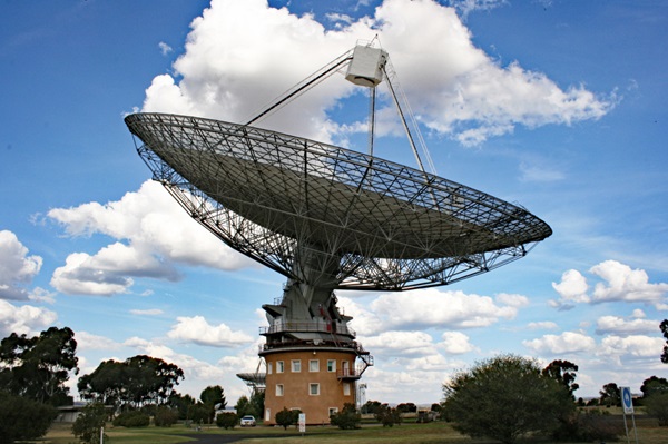
Parkes 64 meter radio telescope in Australia. Courtesy of Bob Naeye and Astronomy.com
The 64-meter Parkes radio telescope in Australia (shown above) detected a faint signal recently while observing Proxima Centauri, a red dwarf 4.25 light-years from Earth. Proxima is visible from the southern hemisphere and is the closest star to our sun. It has at least two planets, one of which is a super-Earth with at least 1.17 Earth masses that orbits in the star’s habitable zone — the region around a star where a planet with the right conditions could host liquid water on its surface. An organization known as “Breakthrough Listen” piggybacks on science observations with the Parkes telescope to simultaneously search for alien signals. Currently the Breakthrough Listen Project is the most advanced SETI (Search for Extraterrestrial Intelligence) endeavor. “Although the press reports are a bit unclear on exactly how and when Parkes detected the signal, it apparently showed up during five 30-minute periods over several days, all while the telescope was pointing directly at Proxima. Notably, when the telescope was turned away from the star, the signal vanished. Ultimately, the signal’s origin appears tightly constrained within a 16′-wide circle — roughly half the size of the Full Moon — around Proxima Centauri on the sky. Breakthrough Listen employs software filters that reject the cacophony of signals originating from Earth or Earth-orbiting satellites to isolate those coming from deep space. But this transmission was unlike anything the project has previously encountered. “.(Astronomy.com). Despite all of this though, the most promising “candidate” for a legitimate call from another civilization in over 40 years is only considered by the project scientists to have a .01% chance that it is the real deal. More than likely it is coming from something on Earth not yet identified.
Arecibo Observatory, Puerto Rico. The Arecibo main radio telescope dish is shown.
Years ago many astronomy enthusiasts here in the US including myself participated in a citizen science project under the direction of the SETI Institute. Data recorded by the mammoth 305 meter radio telescope at Arecibo in Puerto Rico was downloaded and processed on our home desktop machines! They just didn’t have enough processing power to do all of it on site so they asked for our help. I thought it would be incredible to possess the actual computer that confirmed the first evidence for alien life! Unfortunately it was not to be.
The Arecibo Observatory’s main instrument was the Arecibo Telescope, a 305 m (1,000 ft) spherical reflector dish built into a natural sinkhole, with a cable-mount steerable receiver and several radar transmitters for emitting signals mounted 150 m (492 ft) above the dish. Completed in 1963, it was the world’s largest single-aperture telescope for 53 years, surpassed in July 2016 by the Five-hundred-meter Aperture Spherical Telescope (FAST) in China (courtesy Wikipedia). The Arecibo Telescope was decommissioned last month after sustaining irreparable structural damage. The good news is the search for extraterrestrial intelligence is still able to be conducted by many state-of-the-art facilities around the world including the Parkes telescope mentioned at the beginning of this post. For now we will have to wait for the final verdict on the new Breakthrough Listen candidate. Perhaps one day soon there will be an announcement similar to what was heard by astronaut Dave Bowman aboard the Discovery-1 spacecraft in the movie “2001 A Space Odyssey”: “Eighteen months ago, the first evidence for intelligent life off the Earth was discovered”. We will see!